Yesterday I read an article from Wired (Spreadsheets Are Hot—and Cranking Out Complex Code) and it seems that spreadsheets are the new black.
That made think about how much do I use it on my everyday tasks and I noticed that I’m quite a heavy user and a good one. So I decided to write about it and I decided to start talking about my most used and loved ones.
Most of time I use spreadsheets to record activities and some numeric values. I’m not a heavy user on math functions or beautiful and elaborated charts. I’ve been playing with data science, but it’s a different activity mostly done using Plotly, Pandas and Python.
I wrote “Google Spreadsheets” despite “Spreadsheets” because I’m not using Excel any longer. Google Spreadsheets have a wider range of functions than Excel and the cloud allows you to run heavier functions without worring if you’ll brick your Excel file.
The most used one
UNIQUE + MATCH
Since I learned UNIQUE + MATCH my life spreadsheets had changed. UNIQUE + MATCH is much better than VLOOKUP and it let you work with a large ammount of data at once.
Tldr: UNIQUE + MATCH let’s you find a value on another sheet using a value/cell as reference.
E.g. You have a list of fruits and their weights in one sheet. On the other sheet, you have the list of the fruits and their prices. With UNIQUE + MATCH you can create a list with the fruits, weight and price, all at once.
Why UNIQUE + MATCH?
- UNIQUE + MATCH is flexible. You can do horizontal/vertical lookups, 2-way lookups, left lookups, case-sensitive lookups and even lookups based on multiple criteria.
- It works on Excel and Google Spreadsheet
INDEX function
“Returns the content of a cell, specified by row and column offset.” (from Google)
Usage: “INDEX(reference, [row], [column])” (row and column are optional)
E.g.: “INDEX(A1:C20, 5, 1)” this function will get value on row 5, column 1 of the reference “A1:C20”. It will get the value from A5.
MATCH function
“Returns the relative position of an item in a range that matches a specified value.” (from Google)
Usage: “MATCH(search_key, range, [search_type])” (search type is optional but it is usually defined)
E.g.: “MATCH(“Sunday”, A2:A9, 0)” this function will search for “Sunday” from cell A2 to cell A9. If, for e.g., “Sunday” is on cell A4, the function will return 3.
Now let the magic happen
When you join this 2 functions together, magic happens.
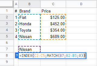
From this example, INDEX select, from C2:C5, the 4th value/row. That happens because MATCH search for Nissan (B7) from B2:B5 and finds that it is on the 4th row. The “0” after “B2:B5” means that I’m looking for an exact MATCH.
Where can I use INDEX + MATCH?
INDEX + MATCH allows you to use Google Spreadsheets or Excel like a small database. When you are working with a lot of data, it’s usually useful to separate it on multiple sheets. E.g.: you have a sheet listing all your contracts and, on another sheet, a list of all your clients. A client may have more than 1 contract with you and if you keep all the data in one sheet, you’ll have to change multiple fields every time that the client info is updated.
You can also use INDEX + MATCH to filter data from a large table where you are looking for a specific data, without the use of the filter function.
You’ll notice that INDEX + MATCH can be applied in many different cases that you need to check and validate data.